Pseudospectral methods

A pseudospectral method represents each state by a polynomial through values at special points called nodes, then enforces the dynamics as equalities at those nodes. This page walks through the LGL (Legendre–Gauss–Lobatto) method used by OpenGoddard.

1. Map time to $[-1,1]$. Use the same reference interval for any phase duration.
2. Place the nodes. Include both endpoints and specially chosen interior points.
3. Interpolate the state. Treat the node values $X_k$ as unknowns.
4. Differentiate with a matrix. Polynomial derivatives are linear combinations of node values.
5. Enforce the dynamics. Match the polynomial slope to the dynamics at every node.
6. Integrate with a weighted sum. Approximate the running cost by quadrature.
7. Solve the NLP. Optimize the node values and phase times with SLSQP.

1. Normalize time

Map $t\in[t_0,t_f]$ linearly to $\tau\in[-1,1]$:

$$t=\frac{t_f-t_0}{2}\tau+\frac{t_f+t_0}{2},\qquad dt=\frac{t_f-t_0}{2}\,d\tau.$$

Thus $dx/dt=2(dx/d\tau)/(t_f-t_0)$. The final time can remain an optimization variable.

2. LGL nodes

For $N$ nodes $\tau_0,\ldots,\tau_{N-1}$, use:

• Endpoints $\tau_0=-1$ and $\tau_{N-1}=1$.
• The $N-2$ roots of $P'_{N-1}(\tau)$ in the interior, where $P_{N-1}$ is a Legendre polynomial.

For $N=5$, the nodes are approximately $-1,-0.6547,0,0.6547,1$. They cluster near the endpoints.

LGL nodes in blue and equally spaced points in gray. As the number of points increases, the LGL nodes cluster more densely near the endpoints.

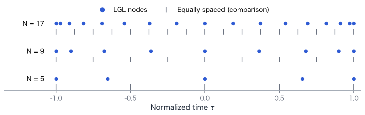
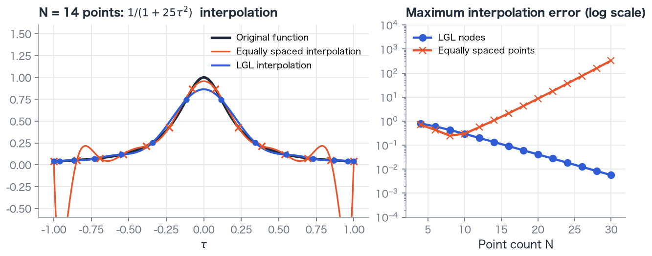
Why not equally spaced points?

High-degree interpolation on equally spaced points can oscillate strongly near the endpoints (Runge’s phenomenon). Adding more points can make the approximation worse. LGL nodes suppress this behavior in the example below and yield rapidly decreasing error.

Interpolation of 1/(1+25τ²) with 14 points (left) and maximum error for different point counts (right, logarithmic scale). Equally spaced interpolation oscillates near the endpoints, while the LGL error decreases rapidly.

How interpolation changes as the number of points increases from 4 to 30.

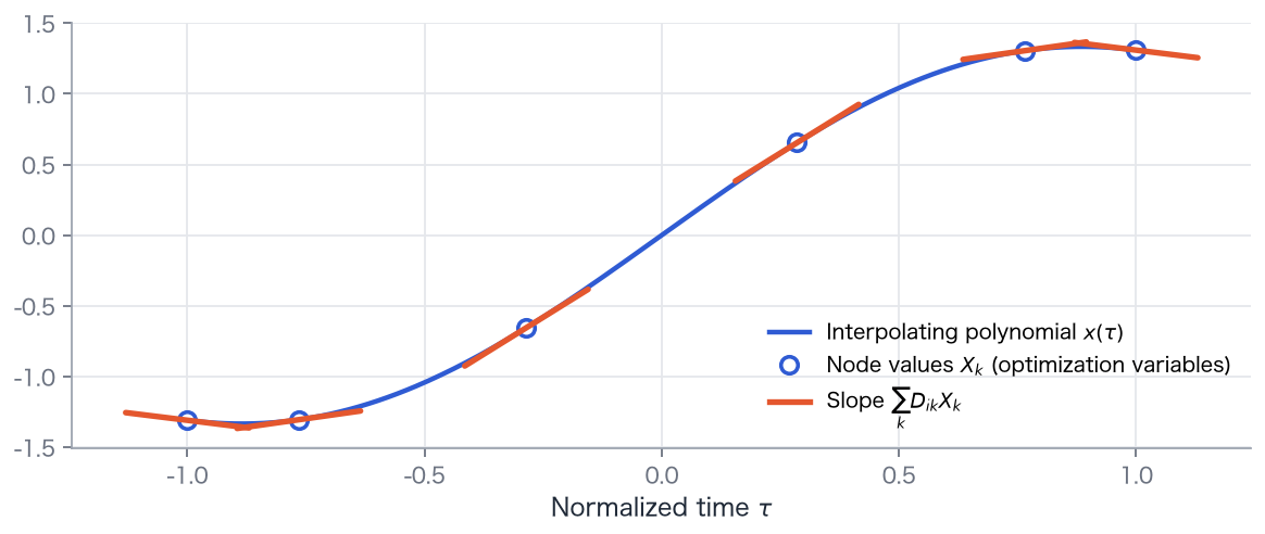
3. Polynomial representation

The node values $X_0,\ldots,X_{N-1}$ are optimization variables. Interpolate them with a polynomial of degree $N-1$:

$$x(\tau)\approx\sum_{k=0}^{N-1}X_k\ell_k(\tau).$$

The Lagrange basis polynomial $\ell_k$ is 1 at $\tau_k$ and 0 at all other nodes. The interpolant therefore takes exactly the value $X_k$ at node $k$. Controls are represented by node values $U_k$ in the same way.

4. Differentiation matrix

The interpolant’s derivative at a node is an exact linear combination of its node values:

$$\left.\frac{dx}{d\tau}\right|_{\tau_i}=\sum_{k=0}^{N-1}D_{ik}X_k,\qquad D_{ik}=\ell'_k(\tau_i).$$

The $N\times N$ differentiation matrix $D$ depends only on node locations and is computed once.

A small example: N = 3

With nodes $-1,0,1$,

$$D=\begin{pmatrix}-\tfrac32&2&-\tfrac12\\[2pt]-\tfrac12&0&\tfrac12\\[2pt]\tfrac12&-2&\tfrac32\end{pmatrix}.$$

For $x(\tau)=\tau^2$, the node values are $X=(1,0,1)$ and

$$DX=\begin{pmatrix}-2\\0\\2\end{pmatrix}.$$

These are exactly the values of $2\tau$ at the nodes. A quadratic is represented exactly by three points, so its derivative is exact too.

A polynomial through six node values (white dots), with slopes computed by the differentiation matrix shown as orange segments. Only the node values are needed to compute the slopes.

5. Enforce the dynamics

Replace $\dot{x}=f(x,u,t)$ by one equality per node, including the time normalization factor:

$$\sum_{k=0}^{N-1}D_{ik}X_k=\frac{t_f-t_0}{2}f(X_i,U_i,t_i),\qquad i=0,\ldots,N-1.$$

The left side is the polynomial slope; the right side is the slope required by the dynamics. Their difference is the defect, which must vanish. Repeat the equations for each state.

Dynamics ẋ = −x. Left: the initial straight-line guess has polynomial slopes (thick blue) that disagree with the dynamics (orange). Right: the solution matches at every node and closely follows e^(−t).

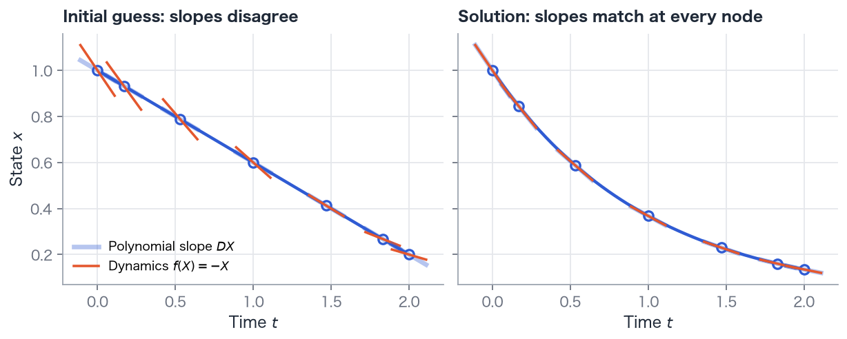
This is the core of direct collocation: handle the differential equation as a set of algebraic slope-matching equations. The optimizer improves the objective while finding node values with zero defects.

6. Quadrature

Use Gauss–Lobatto quadrature for the running cost:

$$\int_{t_0}^{t_f}L\,dt\approx\frac{t_f-t_0}{2}\sum_{k=0}^{N-1}w_kL(X_k,U_k,t_k).$$

The weights depend only on the nodes. This rule is exact for polynomials of degree at most $2N-3$. For $N=3$, $w=(1/3,4/3,1/3)$: Simpson’s rule.

7. Solve the nonlinear program

Collect the unknowns in

$$\boldsymbol{z}=\bigl(\underbrace{X_0,\ldots,X_{N-1}}_{\text{each state}},\underbrace{U_0,\ldots,U_{N-1}}_{\text{each control}},t_f\bigr).$$

The problem becomes

$$\begin{aligned} \min_{\boldsymbol{z}}\quad&\Phi(X_{N-1},t_f)+\frac{t_f-t_0}{2}\sum_kw_kL_k\\ \text{subject to}\quad&DX-\tfrac{t_f-t_0}{2}f(X,U,t)=0&&\text{(defects at each node)}\\ &\psi(X_0,X_{N-1},t_f)=0&&\text{(boundary conditions)}\\ &g(X_k,U_k,t_k)\ge0&&\text{(path constraints)}. \end{aligned}$$

Because LGL includes the endpoints, boundary conditions apply directly to $X_0$ and $X_{N-1}$. For Example 07, three states, one control, and 50 nodes give $50(3+1)+1=201$ unknowns and 150 defect equalities. This scale is practical for SciPy’s SLSQP.

You provide only $f$, $\psi$, $g$, $\Phi$, and $L$. The library computes nodes, differentiation matrices, defects, quadrature, and the NLP.

Multiple phases

A single polynomial cannot accurately represent abrupt thrust switches or mass jumps without oscillating nearby. Split time into phases, each with its own nodes and interpolant, and impose linkage conditions at the knots:

• Continuous states: $X^{(1)}_{\text{last}}=X^{(2)}_{\text{first}}$ (automatic in OpenGoddard).
• Discontinuous states: write the jump yourself, for example $m^{(1)}_{\text{last}}=m^{(2)}_{\text{first}}+\Delta m$.

Goddard thrust histories. Example 07 uses one polynomial and oscillates near burnout. Example 08 splits at burnout, giving a smooth powered phase and exactly zero thrust in the coast phase.

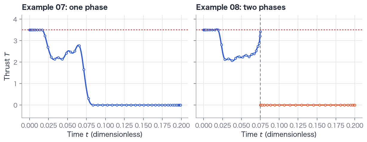
Controls may be discontinuous at knots. Knot times may also be optimized.

Checking accuracy

A successful solver status means that the discretized NLP has been solved. Check whether the trajectory accurately represents the original problem by increasing the node count and comparing results.

Duration error relative to the analytic value √π for Example 03, with different node counts. For smooth solutions, a few additional nodes can reduce the error by many orders of magnitude.

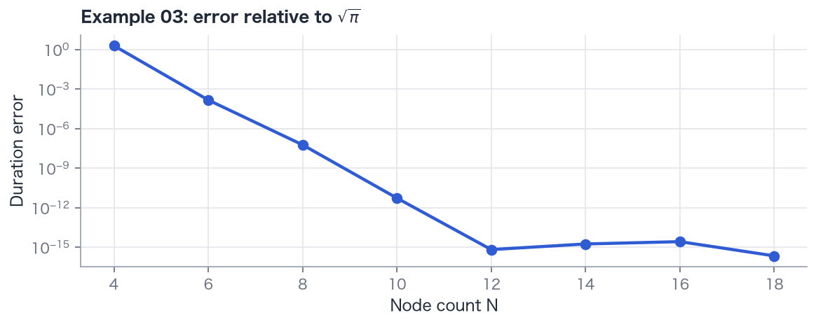
OpenGoddard also provides estimate_error to estimate between-node residuals and solve_adaptive to refine inaccurate phases automatically (writing a problem).

References

Theory and numerical methods

• F. Fahroo and I. M. Ross, “Costate Estimation by a Legendre Pseudospectral Method”, J. Guidance, Control, and Dynamics, 24(2), 2001. doi:10.2514/2.4709
• I. M. Ross and F. Fahroo, “Pseudospectral Knotting Methods for Solving Nonsmooth Optimal Control Problems”, J. Guidance, Control, and Dynamics, 27(3), 2004. doi:10.2514/1.3426
• Q. Gong, F. Fahroo, and I. M. Ross, “Spectral Algorithm for Pseudospectral Methods in Optimal Control”, J. Guidance, Control, and Dynamics, 31(3), 2008. doi:10.2514/1.32908
• A. V. Rao et al., “Algorithm 902: GPOPS, A MATLAB Software for Solving Multiple-Phase Optimal Control Problems Using the Gauss Pseudospectral Method”, ACM Transactions on Mathematical Software, 37(2), Article 22, 2010. doi:10.1145/1731022.1731032
• J. T. Betts, Practical Methods for Optimal Control and Estimation Using Nonlinear Programming, 2nd ed., SIAM, 2010. A standard reference on direct methods.

Launch vehicle trajectory optimization

• I. Ross, C. D’Souza, F. Fahroo, and J. Ross, “A Fast Approach to Multi-Stage Launch Vehicle Trajectory Optimization”, AIAA Guidance, Navigation, and Control Conference and Exhibit, 2003. doi:10.2514/6.2003-5639
• J. R. Rea, “A Legendre Pseudospectral Method for Rapid Optimization of Launch Vehicle Trajectories”, MIT, 2001. MIT repository

Japanese-language references

• Masanori Harada, study of accurate quadrature weights for Jacobi pseudospectral optimization, Transactions of the JSME, Series C, 77(784), pp. 4458–4467, 2011. doi:10.1299/kikaic.77.4458
• Masanori Harada, estimation of dual variables in Jacobi pseudospectral optimal control, Transactions of SICE, 49(8), pp. 808–815, 2013. doi:10.9746/sicetr.49.808
• Masanori Harada, trajectory optimization using high-order Gauss–Lobatto weights in the Jacobi pseudospectral method, Transactions of the JSME, Series C, 73(728), pp. 1075–1080, 2007. doi:10.1299/kikaic.73.1075
• Takahiro Fujikawa, Takeshi Tsuchiya, and Hideyuki Taguchi, hypersonic flight testing using a sounding rocket, part 2: trajectory study, Space Transportation Symposium FY2012 proceedings, 2013. JAXA repository