Numerical approaches

Numerical optimal control methods fall into indirect and direct methods. The distinction is whether we first derive optimality conditions or first approximate the problem with finitely many numbers. OpenGoddard uses a direct pseudospectral method.

	Indirect methods	Direct methods
Approach	Optimize, then discretize	Discretize, then optimize
Resulting problem	Two-point boundary-value problem	Nonlinear programming problem (NLP)
Typical methods	Pontryagin’s minimum principle with shooting	Direct shooting and collocation, including pseudospectral methods

Indirect methods: derive optimality conditions first

Connection to ordinary optimization

At a smooth minimum of $f(x)$, we have $f'(x)=0$. An indirect approach first derives this equation, then solves it. For constrained problems, Lagrange multipliers play the same role.

In optimal control, Pontryagin’s minimum principle introduces time-dependent multipliers $\boldsymbol{\lambda}(t)$ for the dynamics. The Hamiltonian is

$$H(\boldsymbol{x},\boldsymbol{u},\boldsymbol{\lambda},t)=L(\boldsymbol{x},\boldsymbol{u},t)+\boldsymbol{\lambda}^{\top}\boldsymbol{f}(\boldsymbol{x},\boldsymbol{u},t).$$

The multipliers are called costates or adjoint variables. An optimal solution satisfies

$$\begin{aligned} \dot{\boldsymbol{x}}&=\frac{\partial H}{\partial\boldsymbol{\lambda}}=\boldsymbol{f}&&\text{(dynamics)}\\[2pt] \dot{\boldsymbol{\lambda}}&=-\frac{\partial H}{\partial\boldsymbol{x}}&&\text{(costate equations)}\\[2pt] \boldsymbol{u}^{*}(t)&=\operatorname*{arg\,min}_{\boldsymbol{u}}H&&\text{(minimize at each instant)}. \end{aligned}$$

Boundary conditions and terminal costate conditions (transversality conditions) complete the system.

Example: minimum-time move and stop

For $\dot{x}=v$, $\dot{v}=a$, $\lvert a\rvert\le2$ from the preceding page, duration is $\int_0^{t_f}1\,dt$, so $L=1$:

$$H=1+\lambda_xv+\lambda_va.$$

The costate equations give $\dot{\lambda}_x=0$ and $\dot{\lambda}_v=-\lambda_x$. Thus $\lambda_x$ is constant and $\lambda_v$ is linear in time. Minimizing $H$ yields

$$a^{*}(t)=\begin{cases}+2&(\lambda_v(t)<0)\\-2&(\lambda_v(t)>0).\end{cases}$$

A linear function changes sign at most once, so we know in advance that the optimum switches once from maximum acceleration to maximum braking. Revealing the structure of the solution is a major strength of indirect methods.

Two-point boundary-value problems and shooting

The state has a known initial value, but the costate generally has terminal conditions instead. Differential equations with conditions at both ends form a two-point boundary-value problem.

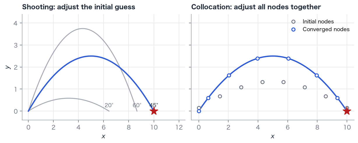
In shooting, guess $\boldsymbol{\lambda}(t_0)$, integrate to the end, measure the terminal mismatch, and adjust the guess. It resembles adjusting a cannon’s aim until it hits a target.

Left: shooting adjusts initial values after integrating to the endpoint. Right: collocation adjusts all node values together to satisfy the dynamics and boundary conditions.

Strengths and limitations

• Strength: high accuracy and analytic insight into the structure, such as the number of switches.
• Limitation: the Hamiltonian and costate equations must be derived for each problem. Inequality constraints can require guessing the sequence of constrained and unconstrained arcs.
• Limitation: costate guesses have little physical intuition. Integration can amplify small errors exponentially, making convergence sensitive to the guess.

Direct methods: discretize first

Represent the unknown functions $\boldsymbol{x}(t)$ and $\boldsymbol{u}(t)$ by finitely many numbers and express the dynamics, constraints, and objective in terms of them:

$$\min_{\boldsymbol{z}}F(\boldsymbol{z})\quad\text{subject to}\quad\boldsymbol{c}(\boldsymbol{z})=\boldsymbol{0},\quad\boldsymbol{d}(\boldsymbol{z})\ge\boldsymbol{0}.$$

This is a nonlinear programming problem (NLP), solvable by a general-purpose optimizer. OpenGoddard defaults to SciPy’s SLSQP, a sequential quadratic programming method that repeatedly solves local approximations with a quadratic objective and linearized constraints.

Direct shooting

Parameterize only the controls, for example as piecewise constants, and obtain the states by numerical integration. This uses fewer variables, but integration can amplify errors, as in indirect shooting.

Collocation

Treat both state and control values at time nodes as unknowns. Replace integration by equality constraints requiring the state derivative to match the dynamics at every node. Optimization improves the objective and enforces the dynamics simultaneously. Avoiding repeated long integrations often makes the method more tolerant of poor initial guesses.

Collocation methods differ in their interpolants:

• Local collocation: use low-degree polynomials on short intervals, as in trapezoidal or Hermite–Simpson methods. These are robust, but accuracy usually improves algebraically with the number of points.
• Global collocation, or pseudospectral methods: use one high-degree polynomial over an entire phase, with specially placed nodes. For smooth solutions, error can decrease exponentially as nodes are added.

Strengths and limitations

• Strength: write dynamics, constraints, and costs without deriving costates or a Hamiltonian.
• Strength: express inequalities directly, without guessing where each constraint is active.
• Strength: initial guesses use physically meaningful states and controls.
• Limitation: more variables, roughly nodes times the number of states and controls.
• Limitation: the result is a local optimum of the discretized problem; accuracy depends on the discretization.

Where pseudospectral methods fit

Pseudospectral methods are direct global collocation methods. Their main advantages are:

1. High accuracy with few nodes. In Example 03, increasing the node count from 6 to 8 to 10 reduces the duration error from roughly $10^{-4}$ to $10^{-7}$ to $10^{-11}$. At 12 nodes it approaches roundoff (accuracy check).
2. Small optimization problems. Relatively few variables make general-purpose solvers such as SLSQP practical.
3. Access to indirect information. NLP multipliers can estimate the continuous costates (Fahroo & Ross, 2001), allowing a direct solution to be checked against the minimum principle.

Discontinuities require care. A single polynomial oscillates near abrupt thrust switches or mass jumps. Split time into phases and use a separate polynomial in each (Examples 07 and 08).

Node choices include LG (Gauss), LGR (Radau), and LGL (Lobatto). OpenGoddard uses LGL, which includes both endpoints, making boundary and linkage conditions straightforward. The next page explains the construction.