01. Minimum-effort transfer

Move a point a fixed distance along a line. Moving faster saves time but requires larger inputs. Moving slowly uses less effort but takes longer. Which motion gives the best balance?

Item	Definition
State	Position $x$
Control	Velocity $u$
Objective	Minimize duration plus the integral of squared velocity
Phases	One phase, 8 nodes, fixed start time 5, free final time
New concepts	Dynamics, boundary conditions, terminal and running costs

Situation

We choose the point’s velocity $u$ at every instant. This input is the control; position $x$, determined by that choice, is the state (terminology). We want to move from $x=0$ to $x=2$ while balancing two goals:

• Arrive sooner.
• Use less effort, measured by the integral of $u^2$.

All quantities are dimensionless. The purpose is to learn the structure of an optimal control problem.

Formulation

Dynamics

$$\dot{x}=u.$$

Position changes at the chosen velocity. This relationship must hold throughout optimization.

Boundary conditions

$$x(t_0)=0,\qquad x(t_f)=2.$$

The start time is fixed at $t_0=5$ to demonstrate that time need not start at zero. The optimal duration does not depend on this offset. The final time is free.

Constraints

$$0\le u\le3,\qquad 5.1\le t_f\le15.$$

Duration therefore lies between 0.1 and 10. Neither bound is active at the optimum.

Objective

$$J=\underbrace{(t_f-t_0)}_{\text{duration}}+\underbrace{\int_{t_0}^{t_f}u^2\,dt}_{\text{control effort}}.$$

The first term is a terminal cost; the second is a running cost. Reducing duration requires faster motion and increases the running cost.

Parameters and scaling

Symbol	Meaning	Value
$d$	Distance (target)	2
$t_0$	Start time	5
$u_{\max}$	Velocity limit	3

The time and position units are 3 and 2 internally (scaling). Results are returned in the original units.

Initial guess

Start with time 5 to 8, position increasing linearly from 0 to 2, and constant velocity $2/3$.

Results

Position and velocity. Dots show the eight nodes, the blue curves are interpolants, black dashed curves are analytic solutions, and the red dotted line is the velocity limit 3.

Motion along the line (left) and position and velocity histories (right). The vertical cursor marks the current time.

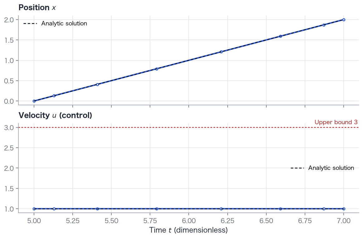
• Duration: 2.0000; objective: 4.0000.
• Velocity remains 1.0000 throughout, and position increases linearly.
• The velocity limit is inactive everywhere.

Explanation

Best motion for a fixed duration

Let $T=t_f-t_0$. The mean velocity is $d/T$. For a given mean, constant velocity minimizes the integral of the square: the mean square is at least the square of the mean. Thus $u=d/T$ and

$$\int_{t_0}^{t_f}u^2\,dt=\left(\frac{d}{T}\right)^2T=\frac{d^2}{T}.$$

Best duration

$$J(T)=T+\frac{d^2}{T}.$$

Setting $dJ/dT=1-d^2/T^2=0$ gives

$$T=d=2,\qquad u=d/T=1,\qquad J=2d=4.$$

The computed duration 2.0000 and objective 4.0000 agree. For this particular objective, the optimal speed is 1 regardless of distance, provided the bounds remain inactive. Only duration changes.

What the numerical method does

OpenGoddard optimizes position and velocity at eight nodes, plus final time, subject to dynamics and constraints (direct methods, pseudospectral methods). The solution is linear in position and constant in velocity, so even eight nodes represent it exactly.

Try it

• Change target = 2.0 in main() to 1 or 5. Duration should equal distance and velocity should remain 1.
• Set target to 20. The unconstrained duration 20 exceeds the allowed duration 10, so the optimum has duration 10, velocity 2, and cost $10+20^2/10=50$.
• Change the node count in Problem([5, 8], [8], ...) to 3 or 20 and compare the answer.

Run

uv run python examples/01_minimum_energy_transfer.py

View the Python source on GitHub.