What is optimal control?

Optimal control finds time-varying inputs that achieve the best objective while satisfying the required conditions. This page introduces each part of a problem through an example, then gives the general mathematical form.

Beyond ordinary optimization

Ordinary optimization might ask for the number $x$ that minimizes $f(x)=(x-1)^2$. The answer is $x=1$. Even with several variables, the unknown is still a finite set of numbers.

Optimal control instead asks for a function of time, $u(t)$: how much to press the accelerator at every instant, for example. Each input also affects later states. Accelerating too hard now may require harder braking later. We must choose the entire input history while accounting for these effects through time.

Example: move and stop in minimum time

Consider Example 02:

Move a cart from rest to a point 10 m away and stop there. Acceleration is limited to 2 m/s² in magnitude. How should acceleration change over time to arrive as soon as possible?

State: the current condition of the system

The state describes the system at a given time. Here it consists of position $x$ and velocity $v$. Together they provide the starting point for predicting future motion. We collect states in a vector $\boldsymbol{x}(t)$.

Control: the input we can choose

The control is the input we are free to choose at each instant: acceleration $a$ here. Its time history $a(t)$ is what we seek. A vector of controls is written $\boldsymbol{u}(t)$.

Dynamics: how inputs change the state

Differential equations describe how the state evolves:

$$\dot{x}=v,\qquad \dot{v}=a.$$

The dot denotes differentiation with respect to time, $\dot{x}=dx/dt$. In general,

$$\dot{\boldsymbol{x}}(t)=\boldsymbol{f}\bigl(\boldsymbol{x}(t),\boldsymbol{u}(t),t\bigr).$$

For a rocket, $\boldsymbol{f}$ includes thrust, drag, gravity, and propellant consumption. The dynamics are constraints that the solution must obey: an advantageous trajectory is unusable if it violates the physical model.

Boundary conditions: the start and finish

Boundary conditions specify the state at the endpoints:

$$x(0)=0,\quad v(0)=0,\qquad x(t_f)=10,\quad v(t_f)=0.$$

The final time $t_f$ is often unknown and determined as part of the solution, as in this example.

Path constraints: limits along the way

Path constraints must hold throughout the motion. Here,

$$-2\le a(t)\le 2.$$

Other examples include maximum thrust, acceleration below 8 G, or altitude above the ground.

Objective: what to improve

The objective function, also called the cost function, expresses what to minimize. Here it is simply arrival time:

$$J=t_f.$$

To maximize a quantity such as final altitude, minimize its negative.

The answer

Apply maximum acceleration during the first half, then switch to maximum braking at the midpoint. The duration is $2\sqrt{10/2}=4.47$ s. OpenGoddard recovers this result numerically.

Example 02: position, velocity, and acceleration. Dots are optimized node values; black dashed curves are the analytic solution. A control that switches between its upper and lower bounds is called bang-bang control.

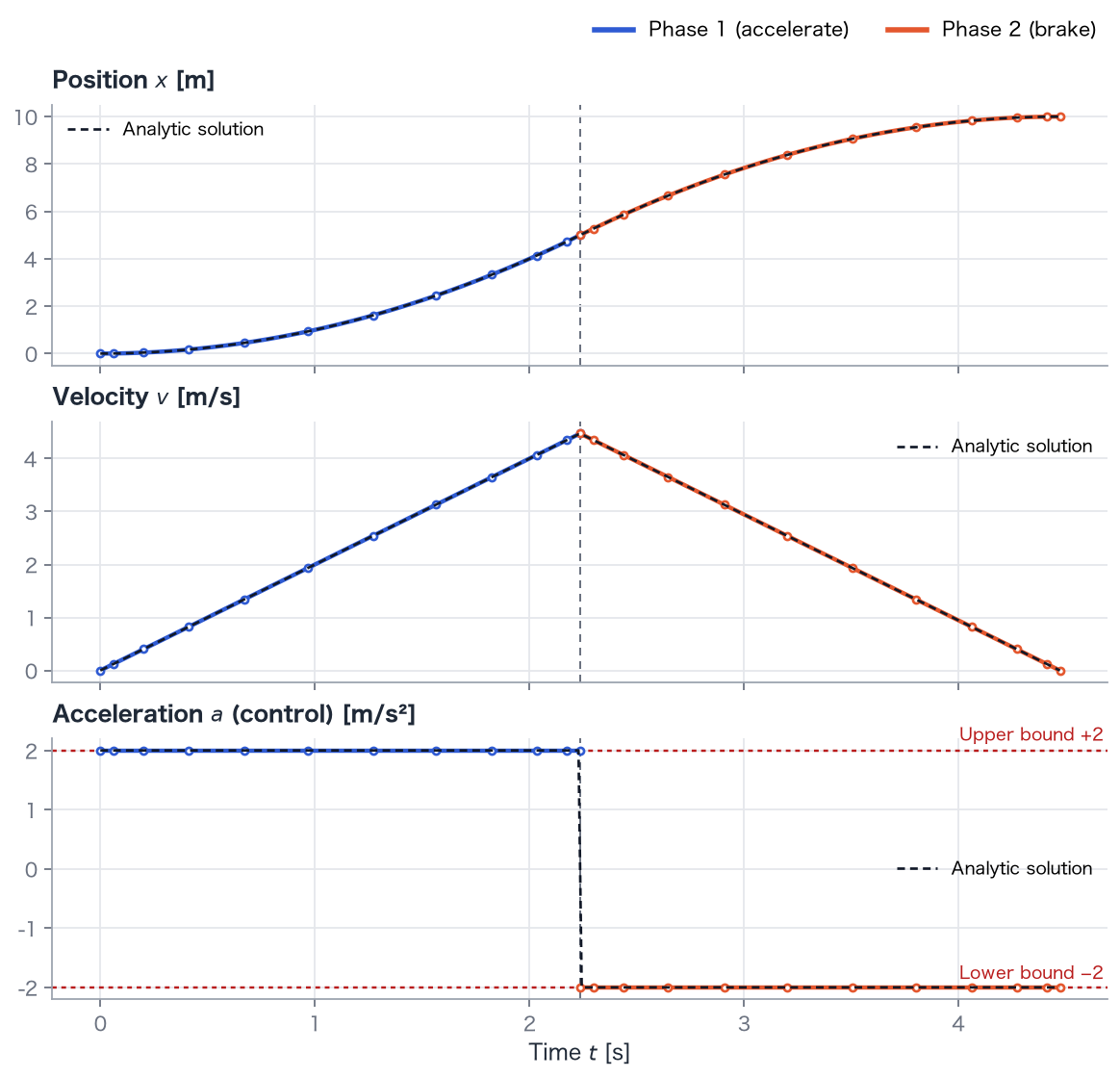
This answer is intuitive, but adding drag, propellant consumption, or altitude-dependent air density soon makes a hand calculation impractical. OpenGoddard solves such problems numerically.

Two forms of cost

Type	Form	Meaning	Examples
Terminal cost (Mayer)	$\Phi(\boldsymbol{x}(t_f),t_f)$	Depends on the final state and time	$t_f$, $-h(t_f)$, $-m(t_f)$
Running cost (Lagrange)	$\displaystyle\int_{t_0}^{t_f}L(\boldsymbol{x},\boldsymbol{u},t)\,dt$	Accumulates along the trajectory	$\int u^2dt$, $\int\lvert T\rvert dt$

Their sum is the Bolza form. Example 01 balances shorter travel time against a larger integral of squared control.

General formulation

$$\begin{aligned} &\text{Minimize} &&J=\Phi\bigl(\boldsymbol{x}(t_f),t_f\bigr)+\int_{t_0}^{t_f}L\bigl(\boldsymbol{x}(t),\boldsymbol{u}(t),t\bigr)\,dt\\[4pt] &\text{Dynamics} &&\dot{\boldsymbol{x}}(t)=\boldsymbol{f}\bigl(\boldsymbol{x}(t),\boldsymbol{u}(t),t\bigr)\\[4pt] &\text{Boundary conditions} &&\boldsymbol{\psi}\bigl(\boldsymbol{x}(t_0),t_0,\boldsymbol{x}(t_f),t_f\bigr)=\boldsymbol{0}\\[4pt] &\text{Path constraints} &&\boldsymbol{g}\bigl(\boldsymbol{x}(t),\boldsymbol{u}(t),t\bigr)\ge\boldsymbol{0} \end{aligned}$$

Symbol	Meaning	In Example 02
$\boldsymbol{x}(t)$	State	$(x,v)$
$\boldsymbol{u}(t)$	Control	$a$
$\boldsymbol{f}$	Dynamics right-hand side	$(v,a)$
$\Phi$	Terminal cost	$t_f$
$L$	Running cost integrand	$0$
$\boldsymbol{\psi}=\boldsymbol{0}$	Boundary conditions	$x(0)=0,\ v(0)=0,\ x(t_f)-10=0,\ v(t_f)=0$
$\boldsymbol{g}\ge\boldsymbol{0}$	Path constraints	$2-a\ge0,\ a+2\ge0$

Write inequalities in the $\ge0$ direction: $a\le2$ becomes $2-a\ge0$. OpenGoddard follows the same convention (writing a problem).

Multiple phases

Some systems change during a trajectory, such as a rocket at stage separation. Divide time into phases and provide dynamics for each. At the boundaries, impose linkage conditions: position and velocity remain continuous, while mass drops by the discarded stage mass. OpenGoddard supports any number of phases (Example 11).

Why numerical methods?

A function contains infinitely many values. Analytic solutions are available mainly for simple dynamics and few constraints, as in Examples 01–03. For practical problems, approximate these functions with finitely many numbers and solve the resulting computational problem. The next page introduces the two main approaches to this conversion.